Max-flow problem instances in vision
From Computer Vision at Western
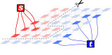
Many optimisation techniques in vision use s-t minimum cuts—either directly or as internal subproblems—and their overall performance relies on efficient maximum flow computation. We host a number of problem instances intended for benchmarking max-flow implementations. The datasets below are representative of typical max-flow problems in computer vision, graphics, and biomedical image analysis.
Contents |
Problem format
A maximum flow problem instance is defined by
- a capacitated digraph
 , with non-negative arc capacities
  , and
, and
- distinct vertices
 designated the source and the sink respectively.
All instances are given in DIMACS format (.max) and maximum flow values are given in corresponding DIMACS solution files (.sol).
| Note. | When applicable, our DIMACS files contain 'hints' indicating repetitive graph structure. This is for the benefit of specialised max-flow implementations. See our graph regularity DIMACS conventions for details. |
Stereo instances
Stereo problem instances below are mirrored from V. Kolmogorov's page. Two types of graphs are constructed based on the papers:
- [BVZ] Markov Random Fields with Efficient Approximations. Yuri Boykov, Olga Veksler and Ramin Zabih. In Computer Vision and Pattern Recognition (CVPR), June 1998.
- [KZ2] Computing Visual Correspondence with Occlusions using Graph Cuts. Vladimir Kolmogorov and Ramin Zabih. In International Conference on Computer Vision (ICCV), July 2001.
Each download contains a sequence of max-flow instances that must be solved by the α-expansion algorithm [BVZ]. This means that each sequence corresponds to the subproblems generated by the first iteration only of α-expansion. In this application it is possible for instances to have no connections to source or sink. The measure of efficiency should be based on total time for each sequence of cuts (tsukuba, sawtooth, venus). Extract each download with tar -xvjf <file>.
- BVZ – 4-connected grid w/ dense terminal arcs from source or to sink.
- BVZ-tsukuba.tbz2 (24MB)
- BVZ-sawtooth.tbz2 (49MB)
- BVZ-venus.tbz2 (44MB)
- KZ2 – two 4-connected grids w/ sparse connections between them (each vertex is connected to at most two vertices in the other grid); dense terminal arcs from source or to sink.
- KZ2-tsukuba.tbz2 (63MB)
- KZ2-sawtooth.tbz2 (119MB)
- KZ2-venus.tbz2 (133MB)
The tsukuba photo set provided by Tsukuba University. The sawtooth, venus photo sets are from Middlebury Stereo Benchmark.
Segmentation instances
Segmentation problem instances are provided to compare effects of graph size, neighbourhood size, length of  paths, regional arc consistency (noise), and arc capacity magnitude. The graph construction is described in the papers:
- [BJ01] Interactive Graph Cuts for Optimal Boundary & Region Segmentation of Objects in N-D images. Yuri Boykov, Marie-Pierre Jolly. In International Conference on Computer Vision (ICCV), 1:105-112, 2001.
- [BF06] Graph Cuts and Efficient N-D Image Segmentation. Yuri Boykov, Gareth Funka-Lea. In International Journal of Computer Vision (IJCV), 70(2):109-131, 2006.
- [BK03] Computing Geodesics and Minimal Surfaces via Graph Cuts. Yuri Boykov, Vladimir Kolmogorov. In International Conference on Computer Vision (ICCV), 1:26-33, 2003.
Extract each download with tar -xvjf <file>.

- liver – 128×128×119, short paths.
- liver.n6c10.tbz2 (94MB) – 6-connected, max capacity 10
- liver.n6c100.tbz2 (102MB) – 6-connected, max capacity 100
- liver.n26c10.tbz2 (270MB) – 26-connected, max capacity 10
- liver.n26c100.tbz2 (281MB) – 26-connected, max capacity 100

- adhead – 256×256×192, long paths (s connected to interior, boundary connected to t).
- adhead.n6c10.tbz2 (254MB) – 6-connected, max capacity 10
- adhead.n6c100.tbz2 (284MB) – 6-connected, max capacity 100
- adhead.n26c10.tbz2 (988MB) – 26-connected, max capacity 10
- adhead.n26c100.tbz2 (1,021MB) – 26-connected, max capacity 100

- babyface – 250×250×81, 'noisy' arc capacities (based on ultrasound data).
- babyface.n6c10.tbz2 (95MB) – 6-connected, max capacity 10
- babyface.n6c100.tbz2 (100MB) – 6-connected, max capacity 100
- babyface.n26c10.tbz2 (350MB) – 26-connected, max capacity 10
- babyface.n26c100.tbz2 (371MB) – 26-connected, max capacity 100

- bone – each download comes with 6 versions of different size but with essentially the same seeds/cut and 'difficulty' relative to problem scale.
- bone.n6c10.tbz2 (303MB) – 6-connected, max capacity 10
- bone.n6c100.tbz2 (341MB) – 6-connected, max capacity 100
- bone.n26c10.tbz2 (1,192MB) – 26-connected, max capacity 10
- bone.n26c100.tbz2 (1,226MB) – 26-connected, max capacity 100
- The sizes scale down by a factor of two at each step, and are called:
bone (256×256×119) bone_subxyz (128×128×60) bone_subx (128×256×119) bone_subxyz_subx (64×128×60) bone_subxy (128×128×119) bone_subxyz_subxy (64×64×60)

- abdomen_long – 512×512×551, very long paths, longer on t side of cut. Source is connected to center of object, boundary is connected to sink. Compare abdomen_short.
- abdomen_long.n6c10.tbz2 (3,166MB) – 6-connected, max capacity 10
- abdomen_short – 512×512×551, same cut as abdomen_long, but short paths on both sides of cut. Voxels just outside the object are connected to sink.
- abdomen_short.n6c10.tbz2 (3,166MB) – 6-connected, max capacity 10
The liver, bone, abdomen, babyface volumetric scans were provided by Siemens Corporate Research; adhead volumetric scan was provided by Robarts Research Institute.
Multiview reconstruction instances
The graph constructions for these multiview datasets are based on a cell complex described in [LB06]. The cut optimises an approximation to the functional described in [BL06].
- [LB06] Oriented Visibility for Multiview Reconstruction. Victor Lempitsky, Yuri Boykov, and Denis Ivanov. In European Conference on Computer Vision (ECCV), LNCS 3953, 3:226-238, May 2006.


- [BL06] From Photohulls to Photoflux Optimization. Yuri Boykov and Victor Lempitsky. In British Machine Vision Conference (BMVC), 3:1149-1158, September 2006.
Extract each download with tar -xvjf <file>.
- BL06-camel – 3D volumetric cut based on 17 photos.
- BL06-camel-sml.tbz2 (25MB) – 40×30×42 grid, 24 oriented cells per grid location.
- BL06-camel-med.tbz2 (199MB) – 80×60×84 grid, 24 oriented cells per grid location.
- BL06-camel-lrg.tbz2 (388MB) – 100×75×105 grid, 24 oriented cells per grid location.
- BL06-gargoyle – 3D volumetric cut based on 15 photos.
- BL06-gargoyle-sml.tbz2 (23MB) – 32×45×32 grid, 24 oriented cells per grid location.
- BL06-gargoyle-med.tbz2 (183MB) – 64×90×64 grid, 24 oriented cells per grid location.
- BL06-gargoyle-lrg.tbz2 (351MB) – 80×112×80 grid, 24 oriented cells per grid location.
The gargoyle photo set provided by Kyros Kutulakos. DIMACS instances and camel photo set provided by Victor Lempitsky.
Surface fitting instances
Shape fitting problem instances are coming soon. The graph construction has particularly short paths, as described in the paper:
- [LB07] Global Optimization for Shape Fitting. Victor Lempitsky and Yuri Boykov. In IEEE Computer Vision and Pattern Recognition (CVPR), June 2007.

Extract each download with tar -xvjf <file>.
- LB07-bunny – 3D volumetric surface fit based on 112 laser scans of the Stanford Bunny.
- LB07-bunny-sml.tbz2 (12MB) – 102×100×79, 6-connected grid.
- LB07-bunny-med.tbz2 (89MB) – 202×199×157, 6-connected grid.
- LB07-bunny-lrg.tbz2 (705MB) – 401×396×312, 6-connected grid.
Dynamic problem instances
Many applications in vision require solving max-flow problem of similar graphs. For example, this happens when an image changes from frame to frame in a video sequence or when solutions are computed for a sequence of nearby locations in an image. Many standard max-flow algorithms can have a "hot start" when solving each new instance by reusing internal data structures. Typically, this significantly speeds up the algorithms compared to independent solution of all instances. Examples of existing dynamic max-flow algorithms are:
- [KT05] Efficiently solving dynamic markov random fields using graph cuts. P. Kohli and P. Torr. In International Conference on Computer Vision (ICCV), 2005.
- [JB06] Active graph cuts. Olivier Juan and Yuri Boykov. In IEEE conference on Computer Vision and Pattern Recognition (CVPR), 2006.
Below we posted several examples of dynamic applications. For each download, the starting graph and flow are given by the .max and .sol files outside the folder 'dynamic'. These files 'dynamic+index.max'(.sol) in the 'dynamic' folder specifies consecutive graph change (flow change) over 'dynamic+index-1.max'(.sol). Notice that we give new arc capacities for changed arcs, not incremental capacities.
Part 1 Shape matching
These dynamic maxflow graph instances are based on the shape matching application described in [TGVB13].
- [TGVB13] GrabCut in One Cut. Meng Tang and Lena Gorelick and Olga Veksler and Yuri Boykov. In International Conference on Computer Vision (ICCV), 2013.

Extract download with tar -xvjf <file>.
- TGVB-car – shape matching with a car template.
- TGVB_car_16bins.tbz2 (7MB) – 8 connected neighbor, color separation of 16 bins per channel.
- TGVB_car_32bins.tbz2 (7MB) – 8 connected neighbor, color separation of 32 bins per channel.
- TGVB_car_64bins.tbz2 (7MB) – 8 connected neighbor, color separation of 64 bins per channel.

- TGVB-person – shape matching with a polygon template.
- TGVB_person_16bins.tbz2 (35MB) – 8 connected neighbor, 16 color bins per channel.
- TGVB_person_32bins.tbz2 (35MB) – 8 connected neighbor, 32 color bins per channel.
- TGVB_person_64bins.tbz2 (35MB) – 8 connected neighbor, 64 color bins per channel.
An example of timing for solving these dynamic instances with dynamic max-flow [KT05] and 'static' max-flow [BK04] can be found here. The number of graphs vs time plot is generated for TGVB_person_64bins instance.
- [BK04] An experimental comparison of min-cut/max-flow algorithms for energy minimization in vision. Yuri Boykov and Vladimir Kolmogorov. In IEEE transactions on Pattern Analysis and Machine Intelligence (PAMI), 26(9):1124-1137, 2004.
Part 2 Video segmentation
These graphs are constructed based on image and video segmentation described in [BJ01] and [KT05].

- VideoSeg – video segmentation with fixed appearance models
- VideoSegA.rar (129MB) – 8 connected neighbor.
- VideoSegA2.rar (129MB) – 8 connected neighbor, extra temporal consistency on SegA.
- VideoSegB.rar (71MB) – 8 connected neighbor.
- VideoSegB2.rar (71MB) – 8 connected neighbor, extra temporal consistency on SegB.
An example of timing for solving these dynamic instances with dynamic max-flow [KT05] and 'static' max-flow [BK04] can be found here. The number of frames vs time plot is generated for VideoSegB2 instance.
Video credit: youtube source
Part 3 One-Cut Video segmentation
These dynamic max-flow graph instances render energy consisting of spacial regularization term, L1 color separation term [TGVB13] and L2 temporal consistency term between two consecutive video frames. Appearance model prior is not provided for these instances.
Not only are edge capacities changing in these instances, but also graph structures vary over time. These challenging dynamic graphs benefit from more powerful dynamic maxflow algorithms.
For each download, if new arc capacity is zero, then it means the two vertexes adjacent to the arc are disconnected.


- OneCutVideoSeg – video segmentation with color separation term [TGVB13]
- VideoSegA3.rar (161MB)
- VideoSegB3.rar (114MB)
- VideoSegC.rar (205MB)
- VideoSegD.rar (245MB)
video credit: Freiburg-Berkeley Motion Segmentation Dataset